Lab 5: Image Mosaic and Other Functions

Introduction:

This lab was designed to help teach and explore image mosaic, spatial and spectral image enhancement, band ratio, and binary change detection.  All of these functions are key in understanding how to best use ERDAS to aid in imagery interpretation and practical applications of remote sensing analysis.

Methods:

Image Mosaicking: 

Image mosaic is taking several separate scenes of satellite imagery and processing them into one seamless scene.  It is performed when a desired study area is larger than the spatial extent of a given satellite image scene.  It is also useful when the area of interest covers the portion of two intersected satellite scenes.  The first portion of this lab involved looking at two satellite images of the Eau Claire area together in the same viewer (Figure 1).  This produced what was clearly two contiguous, but separate satellite images.

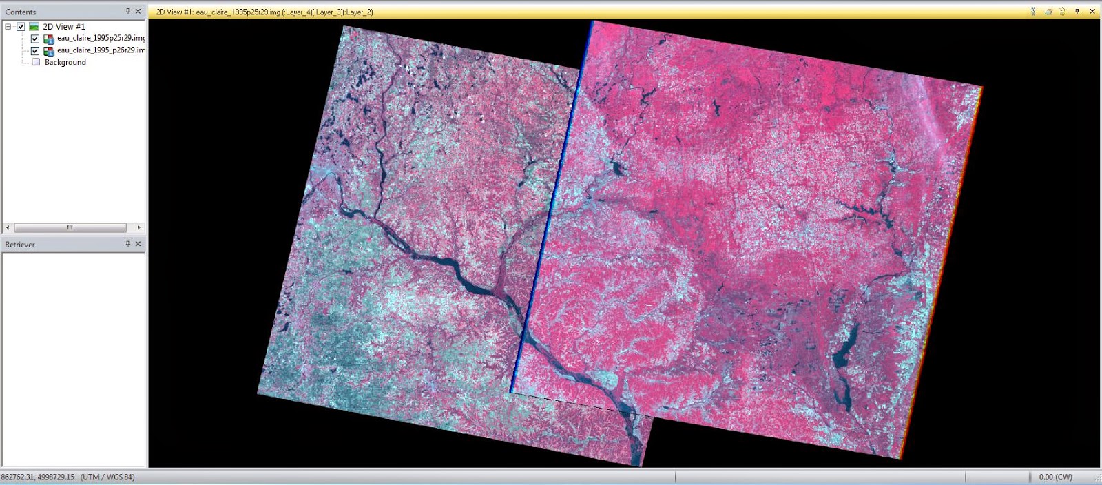As can be clearly seen, the displaying of the two satellite images on top of each other, even though they are contiguous, isn't very advantageous for visual interpretation. (Figure 1) 

From here, the images were mosaicked using a tool called Mosaic Express (Figure 2) under the Raster menu.  Which produced an output that looked almost less useful than the original two separate images (Figure 3).

Mosaic Express is under the Raster menu and is a quick and easy way to mosaic imagery together. (Figure 2)

Mosaic Express produced this seamed together image which unfortunately has a large amount of difference between the two images still even though they now are one. (Figure 3)

MosaicPro (Figure 4), another option to mosaic images together was tried next with much more ascetically pleasing results (Figure 5) thanks to histogram matching, which MosaicPro allows.

This is the MosaicPro window.  It is much more complicated then Mosaic Express, but this allows the use of more tools.  Overall it is a more powerful and useful image mosaic option. (Figure 4)

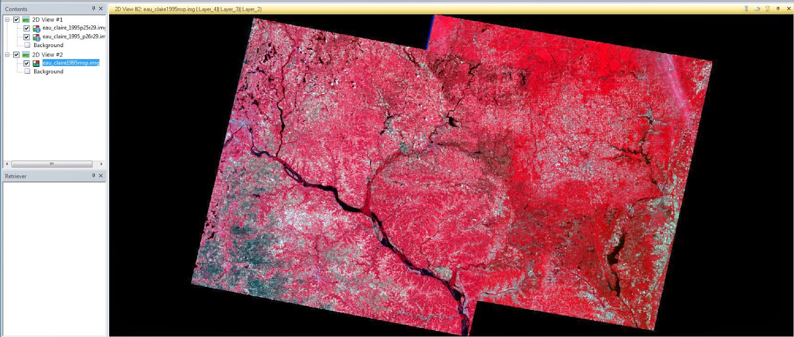This is the final output after MosaicPro was run.  The histogram matching option of MosaicPro helps eliminate the border between the two original input images and allows for better visual interpretation of the whole image using color. (Figure 5)

Band Ratioing:

Band ratioing allows for interpreting of images using reflectance properties.  In this lab NDVI (Normalized Difference Vegetation Index) is looked at in order to analyze vegetation amount in the Eau Claire area.  NDVI can be run in ERDAS under the Raster menu (Figure 6).  Running this tool on a LANDSAT image of the area produced a black and white image (Figure 7), with the brighter areas representing larger amounts of vegetation.

This is the Indices tool with NDVI set as the index.  An image can be input here and it will output an image that displays vegetation concentration. (Figure 6)

This is the NDVI image created from a LANDSAT image of the Minneapolis-Eau Claire area.  The brighter areas represent areas of high vegetation concentration, the darker gray areas mostly represent urban areas, and the black areas represent water in this image. (Figure 7)

Spatial Enhancement:

Spatial enhancement involves adjusting the frequency of an image (how much the pixel value changes over a distance).  The images can be adjust to have a lower frequency or a higher frequency depending on what is desired.  High frequency images (Figure 8) have a high amount of change in a small area of pixels.  The frequency can be lowered using the Convolution tool (Figure 9) in ERDAS.  Similarly, low frequency images can have their frequency raised to appear less blotchy.

This is a satellite image of Chicago.  It has a high frequency, which makes it appear too busy in some areas which can hamper visual image analysis. (Figure 8)

This is an image of the Convolution tool in ERDAS.  As can be seen, Low Pass is selected which will lower the frequency of an image. (Figure 9)

Spectral Enhancement:

Spectral enhancement involves stretching out the histogram of an image in order to give the image a larger contrast.  This can be done using many different methods.  Usually the method of stretching out the histogram depends on input histogram mode.  Gaussian histograms, or histograms with one peak, are typically stretched using a maximum-minimum contrast stretch (Figure 10).  This type of contrast stretch simply pulls out the max and min of the histogram to values of 0 and 255.  Non-Gaussian histograms, histograms with multiple peaks) can be stretched out in a piecewise contrast stretch (Figure 11).

This image has had it's histogram stretched using a maximum-minimum contrast method, which is best suited for Gaussian histograms. (Figure 10)

This image has been piecewise contrast stretched. (Figure 11)

Histogram Equalization:

Histogram equalization can be done to improve the contrast of an image (Figure 12 and Figure 13).  It aides greatly in visual interpretation if the image has no contrast and has a histogram that's very concentrated in one area.

The left image is the input image, while the right image is the output image which has been run through histogram equalization. (Figure 12)

The left histogram is extremely concentrated and doesn't show much contrast.  However, the right histogram is the output histogram after histogram equalization has been run.  As can be seen, it covers much more area so it, in turn, has a higher contrast. (Figure 13)

Binary Change Detection:

By analyzing the brightness of pixels in a similar image taken at different times, it can be seen if any change has occurred.  Two inputs (Figure 14) can be run through a tool and have their brightness values subtracted from each other.  In this way, the change in brightness values can be detected and an output image can be created (Figure 15).  This can also be done using a model in Model Builder (Figure 16).  This image can have its histogram analyzed and the areas of change can be found by separating different areas on the histogram from each other depending on the pixel value.  In this case, the portions of the histogram that were found to have changed were less than -25.3 and greater than 71.3 (Figure 17).

The left image is an image from 1991 of the Eau Claire area while the one on the right is of the same are from 2011.  The pixel values of band 4 of the 1991 image were then subtracted from the pixel values of band 4 of the 2011 image.      (Figure 14)

This is the output image that was created by subtracting the two input image pixel values.  This image itself doesn't readily show the change from one year to the other.  Instead the histogram needs to be evaluated. (Figure 15)

Running a model using Model Builder is one way to run equations such as subtracting pixel values.  (Figure 16)

This is a histogram of the output image in Figure 15.  The thresholds of change are pixels with values less than -25.3 and greater than 71.3.  These areas are where pixel values changes in brightness from 1991 to 2011. (Figure 17)

From here, another model can be run to give all pixel values that haven't changed a 0 value and all pixel values that have changed a value of 1.  In this way, it can be seen exactly where there was change by looking at the output image.  This image can then be brought into ArcMap (Figure 18).

This map shows the areas where the pixel values changed between 1991 and 2011 near Eau Claire, WI.  (Figure 18)

Conclusion:

This lab taught many useful functions for processing images.  These functions, when used correctly, are extremely powerful in aiding visual image interpretation.  These functions can also be used to solve a problem or answer a question such as:  Where is the vegetation greatest using NDVI, or where has the most change occurred in the Eau Claire region over the last 20 years using binary change detection.  In a well-trained user's hands, it's obvious that ERDAS and these image functions can be used to answer many diverse questions and issues.